IBM Put PCM at Core of Hyperdimensional Computing

By Jim Handy, The Memory Guide, leader, Gerson Lehrman Group, on the advisory board of Flash Memory Summit, written on September 17, 2020

Our PCM maven Ron Neale explored how PCM is being used to benefit AI and ML applications. Although AI is a new spin to The Memory Guy blog, there is a striking similarity between memory chips and certain AI applications, most particularly neural networks.

In this post Neale delves into a recent piece of IBM research published in Nature Electronics, that uses Hyperdimensional Computing algorithms to simplify not only inference, but training as well.  The approach overcomes the sensitivities of neural networks and vastly simplifies training while eliminating wear issues by writing to memory only once even though the memory size is very small.

Neale takes a difficult subject and brings it to a level that can be approached even by those many members of the technical community who are not well versed in AI.

Introduction
A recent paper from IBM, Zurich, Switzerland, published in Nature Communications ^[1] invites us to visit the further progress and success that, partnered with ETH, Zurich, they have achieved in applying phase change memory (PCM) and in-memory computation to the problems of: Language classification, News classification and Hand signals, using what are described as Hyperdimensional Computing (HDC) techniques. The paper provides supporting evidence that PCM-based solutions are equal to, or in some metrics more efficient than, conventional methods.

In the past IBM have applied the special characteristics of PCM which allow in-memory functions of multiplication and addition to solve the problems of compressed sensing (CS) and recovery of sparse signals as well as image reconstruction ^[2], ^[3].

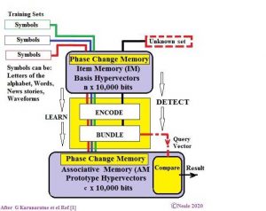
This latest work builds on that earlier work with a complete system which could be considered as a 3-computer stack, where the PCM serves in dual role of computer and memory as illustrated below.

At the core of the process of recognition or inference, be it of characters, words, waveforms or the like, is the magic of linear algebra, where the use of very high-dimensional vectors (10,000 bits) allow clearly separated parking places to be found in multi-dimensional vector space for classes, that is, collections of objects and their subtle differences.

A small sample belonging to an unknown class, can then use the same PCM-based process to find the unique place in multi-dimension vector space allocated for the family or class and effect a successful identification without risk of confusion.

In the diagram above, the system is trained using a range of training sets, identified with red, blue, and green colours. The example we will use in this article will be different languages, and the training set for each language is made up of large text files for each of several languages.  Once the system has been trained, then the unknown set on the top right, which, in this case, could be a short string of text in one of these languages, can be processed to determine its language.

The 2 purple boxes represent the phase change memories (PCMs) in which in-memory processing is performed. This top memory is called the Item Memory and it stores Basis Hypervectors. The bottom memory is called the Associative Memory and it stores Prototype Hypervectors. Between these two is a yellow logic block which performs a task called Bundling.  All of these will be explained later on in this blog post.

The short explanation of the diagram is that a process is performed on each of the training sets via the in-memory processing and Bundling, and the results of this process are stored in the Associative Memory at the bottom.  Now that the system has been trained, an unknown set can be put through the same process and compared within the Associative Memory against the other sets to determine which is the best match.

The use of 10,000-bit words, also called vectors, gives rise to the prefix ‘Hyper’ for Hyperdimensional Computing (HDC) as the description of the approach used in this system.

Hyperdimensional Computing
Hyperdimensional Computing is not new and the algebra and complex probabilistic mathematics already has a place in machine learning and recognition; similar techniques have also been used in digital communications. In fact, robustness of the system in many ways models the operation of the brain and its roots can be found in that literature, all of which requires a large conventional computation overhead.

What is new is a demonstration at the systems level of the ability of the PCM to provide in-memory computation to ease the overall computational work-load, further aided by some IBM innovative vector processing short-cuts.

The memory takes on its normal role as a storage device and that of a computer. PCMs allow the simple application of Ohm’s Law for multiplication and Kirchhoff’s Law for addition to perform complex statistical computation. The resistance of a PCM when subjected to input voltage provides the product in the form of a current (I =V x 1/R) and when a number of PCM cells are connected to a common point the output is the sum of the input currents. Neural networks are often implemented this way.  That is the easy part of PCM-based HDC. From there forward it gets rather more complex and moves into a world of multi-dimensional hypervector space.

Prior implementations of HDC recognition required frequent updates of memory locations, leading to concerns of wear in non-volatile memory-based systems. The IBM research team was able to find mathematical work-arounds that limit all memory locations to be written to only once. All subsequent memory accesses are reads. Furthermore, training and recognition are both performed in a single pass, reducing power consumption while increasing speed.

Another benefit of the HDC approach is its use of extremely simple math in which all operands consist of a single bit. An enormous abundance of operands makes up for this lack of any single operand’s precision. It’s somewhat similar to the way that a quality grey-scale photograph can be made up from a very large collection of tiny black and white dots. Even if some dots go missing the picture is still recognizable. We will see later on how one of this system’s two memories performs functions relatively similar to those of a neural network, but by using single-bit precision rather than multi-bit storage elements the system becomes much less sensitive to variations in the bit cell’s performance.

PCM Device Structures
As a PCM specialist I was naturally interested in learning what kind of PCM IBM used in this design.

The memory arrays used for this latest work each contain 3 million PCM cells and are the same as those used by IBM for their earlier in-memory computing demonstrations. The active memory material is doped Ge₂Sb₂Te₅ (d-GST) with the PCM cells fabricated on 90nm CMOS technology, employing what is described as the ‘keyhole’ process.

The bottom electrode has a radius of 20nm, the d-GST is 100nm thick with an upper electrode radius of 100nm.

It does not appear that IBM have any plans to make their PCM arrays available to third parties in the form of a memory product. Those wishing to apply the hyperdimensional computing techniques will for the moment have to rely on other sources and even other NVM technologies such as ReRAM or MRAM resistance devices.

Simple Problem
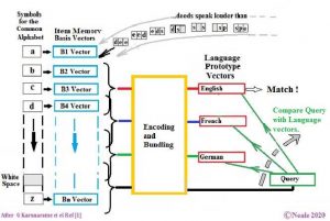
Let us look at the simplest of problems the IBM team solved. Which is analysing a sample of words (including spaces) in the form of a short sentence and identifying the language to which it belongs. For this simplification we will assume the languages all use a similar alphabet. The complete flow diagram for solving that particular problem is illustrated below.

This diagram describes a processing sequence that encapsulates the special characteristics of each language into a single 10,000-element vector. The characteristics in this experiment are the grouping of letters that are peculiar to each language. (For example, English uses the combination ‘th’ more than French or German, while French includes many more instances of ‘qu’ and German more ‘ch’ than the others.)

A stream of characters is input at the top: ‘Deeds speak louder than words.’ The system has been designed to analyse groups of letters so the diagram shows the letters in this string in groups of three.

I will briefly explain the chart using a number of buzzwords that will be defined later on in the text.

Each letter acts as the address for a memory that contains ‘Basis Hypervectors’. The current letter’s Basis Hypervector is combined with the Basis Hypervectors for the other letters in the group, and this combination is sent to the encoding and Bundling mechanism. All of the 3-letter combinations are then Bundled (defined below) into ‘Prototype Hypervectors’ to be stored in the ‘Associative Memory’.

The 10,000-element Prototype Hypervector has no numerical value – it is more the pattern of elements (bits) which carry the information. More accurately, it represents a unique and distinctly separate point in multi-dimensional space. The high number of dimensions means that, during the identification step, some parts of the pattern can be missing from the sample that needs to be identified while still allowing a rapid and accurate identification.

After the system has been trained then a string of text in an unknown language can be processed the same way that the training text was, to generate a ‘Query Hypervector’. This Query Hypervector is then compared against all of the Prototype Hypervectors, to determine which Prototype Hypervector is most similar to the query.

Step-By-Step Functionality
The first step in the move into multi-dimensional vector space involves the creation of what are called the ‘Basis Hypervectors’. The 10,000-bit Basis Hypervectors are required to be random series of equal numbers of ones and zeros to support Hyperdimensional Computing’s unique form of mathematics. They are called Basis Hypervectors because they are the starting point for all of the operations in the device. These Basis Hypervectors are stored in the Item Memory where they remain for the life of the product.

The next step is to create a single ‘Prototype Hypervector’ for each language. Thousands of sentences from each language are analysed to find 3-letter sequences which are a characteristic of a particular language. Every 3-letter sequence in the training text generates a 10,000-bit code based on the Basis Hypervectors. The system has been designed to produce the same 10,000-bit code for every instance of the same three-letter sequence. This code is then added, bit by bit, to the 10,000-bit codes for all of the 3-letter sequences that preceded it. Once the training has been completed these 10,000 sums are tested against a threshold to produce a ‘1’ for numbers above the threshold and a ‘0’ otherwise, resulting in a 10,000-bit Prototype Hypervector unique to that language.

Creating the Prototype Hypervector
Let’s take a look at how this interesting vector is created.

The Basis Hypervectors are loaded into one of the PCM arrays called the Item Memory (IM) as was shown in the first graphic of this post. The Item Memory is configured as N words (the number of letters in the common alphabet, plus a space) each consisting of a 10,000-bit Basis Hypervector, each of which, as previously explained, consists of set of an equal but random number of 1s and 0s. The contents of the Item Memory never change.

As the characters arrive (shown in the arc at the top of the second figure), they each select the appropriate Basis Hypervector, which is then mixed with the Basis Hypervector of the adjacent two letters to form a three-letter group that represents the sequence. The researchers elected to streamline this calculation by using in-memory computing functions. As previously mentioned, the same 10,000-bit code will be generated for every instance of the same three-letter sequence

These sequences for the entire training set are then added in the Bundling mechanism to produce a sum, which is then measured against a threshold to produce the bits of the Prototype Hypervector.  All vectors throughout this process are 10,000 element hypervectors.

One way to think about a language’s Prototype Hypervector is that each bit represents the likelihood that a similarly-generated vector from the same language will have a ‘1’ in that same bit location. That’s because the three-letter groups of that language more commonly generate a hypervector with a ‘1’ in that bit position. If the Prototype Hypervector has a ‘1’ in that bit position then other similarly-generated hypervectors are more likely to have a ‘1’, and if the Prototype Hypervector has a ‘0’ in another bit position then the similarly-generated hypervector is more likely to have a ‘0’ in that position.

The training sequence becomes a single run-through of a large training set. For example, long streams of English text will be run through this process to generate a single English Prototype Hypervector. Once this Prototype Hypervector has been generated it is stored in another PCM memory called the ‘Associative Memory’ in an address which has been set aside to represent the English language. Other addresses will be used to store the Prototype Hypervectors that represent other languages.

This process is then repeated for each language, generating a Prototype Hypervector that represents that language, and storing that language’s Prototype Hypervector into an address in the Associative Memory that has been reserved for that language.

Matching Unknown Text: Query Hypervector
After all of the training languages have been processed the Prototype Hypervectors can be used to determine the language of new text strings. Here’s how:

Although the 10,000-bit Prototype Hypervector appears to be a random distribution of ‘1s’ and ‘0s’, within that vector are statistical patterns unique to the language it represents. If a new text string from the same language is processed the same way as the Prototype Hypervector then it should share similar attributes, although it is unlikely to be identical.

The length of these vectors allows, even if some bits are missing, for a high probability of correctly matching the Prototype Hypervector with the new text string’s hypervector, which is called a ‘Query Hypervector’. It will have been created from a shorter text sequence than the training set, not necessarily containing all sequences or even all letters of the alphabet.

In operation, a text string in an unknown language will be processed into a Query Hypervector. It’s then compared vs. the Prototype Hypervectors for each of the trained languages, and the system determines which is the closest fit. (I’ll explain how next.) The system answers the question: “Which language does this new text string most closely resemble?”

To a large extent the probability of success is enhanced because each language Prototype Hypervector is so remote from the others in multi-dimensional vector space that identification errors are unlikely. The important feature is that the statistical links between the Query Hypervector and the Prototype Hypervector result in a high probability of success when the two are compared.

Matching Queries to Prototypes
The Query Hypervector is matched to a Prototype Hypervector by calculating how close they are to each other in hyperspace. Since all of the dimensions are single-bit variables this calculation is very simple, and boils down to determining how many bits they have in common. The more coincidence there is between ‘1s’and ‘0s’ at each point along the bit strings of the two, the more similar they are to each other.

If the distances were measured in multi-bit values in a space with fewer dimensions then the formal calculation would be quite laborious and would require additional circuit elements. However, because the vectors that are compared have the same number of digits, and since these digits are all binary, IBM have found a neat shortcut, or simplification of the calculation complexity of the distance equations. In essence, hypervectors may have more bits than more conventional approaches, but the math becomes simpler, and that simplicity overshadows the increase in bit count.

As is done with Neural Networks, the Query Hypervector is compared to all of the Prototype Hypervectors by calculating the dot product of the Query and Prototype Hypervectors, which is a one-shot operation. The dot product is the multiplication of the corresponding elements of two vectors followed by the addition of those products.

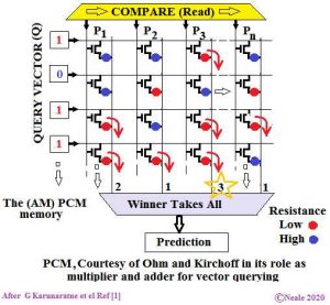
Figure illustrates a small section of the Associative Memory
in which the dot product is performed.

The Query Hypervector is applied to the horizontal lines in this diagram and the Prototype Hypervectors (P1, P2, P3…Pn in the diagram) reside vertically in the PCM bit cells, which are shown as red and blue dots – a red dot represents a low impedance or a ‘1’ and a blue dot represents a high impedance or a ‘0’. Any bit in the Query Hypervector that is a ‘1’ will turn on the transistors in that row. In any bit position in which both the Query Hypervector and the Prototype Hypervector have a ‘1’, both the transistor and the PCM bit cell will allow a current to flow, as indicated by the red arrows, and that current will be fed into the vertical line. This simple action, enabled by Ohm’s Law, performs the multiplication required for the dot products.

Kirchhoff’s Law will then act to provide the sum of the currents on the vertical line, and thus the sum of the products to complete the dot product. The multiplies and adds are performed in a single operation. Different currents are generated in each vertical line, and are denoted at the bottom of each line.  Lines whose Prototype Hypervectors more closely match the incoming Query Hypervector will have higher currents, while other lines will have lower currents.

The yellow box at the top simply sequences through the vertical lines to prevent everything from turning on at once.

Determining which Prototype Hypervector is closest to the Query Hypervector is just a matter deciding which vertical line has the highest current, which is decided by a winner-take-all circuit, with the maximum current confirming the match.

Results
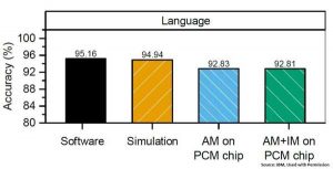
The system provided good accuracy, as illustrated in the chart below, taken from the researchers’ work:

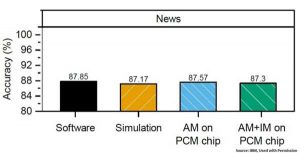
This chart compares 4 different trials: An all-software embodiment of the Hyperdimensional Computing algorithm, a simulation of the PCM-based system, an embodiment in which only the Associative Memory was implemented on the PCM-based chip, and an embodiment in which both the Item Memory and the Associative Memory were implemented on the PCM chip. While the software embodiment was able to use high precision math, it is interesting to see how closely the two PCM implementations came to its performance, even though PCM suffers from internal noise and the currents in the dot products would have been negatively influenced by resistance variations in the PCM bit cells and the select transistors.

Approach worked similarly well in another application which classified news stories

Again, the PCM embodiment compared very favourably against the software embodiment, despite the issues confronted by the hardware.

The researchers estimate that an all-hardware approach using more conventional CMOS, instead of in-memory computing based on PCM, would consume tens to hundreds of times more energy per match and would require a chip tens of times larger area than their design.

A one-shot query method using PCMs which gives the answer without multiple-converging trial-and-error techniques without consuming power and wasting time is a clear advantage of PCM based in-memory computation. The calculation of the dot product with an innovative mixture of PCMs and Ohm’s and Kirchhoff’s Laws provides such a one-shot solution.

In a range of different tests, the PCM-based methodology using in-memory computing proved comparable to conventional all-software-based alternatives in terms of accuracy. For statistical-based systems the result is a prediction and therefore accuracy is one of the metrics of success.

Acknowledgements
I would like to thank Geethan Karunaratne, Manuel Le Gallo, IBM, Zurich, and WebEx for allowing me to cyber-invade their homes and enable them to act as my very patient guides though PCM-driven hypervector hyperdimensional computing space while this article was in preparation, in the Covid-19 infested world of 2020.

References
[1] In-memory hyperdimensional computing, by Geethan Karunaratne, Manuel Le Gallo, et al.  (Ref [1] is long and detailed paper, in this initial review I have of necessity simplified many points and highlighted one innovative circuit detail from many.)
[2] Temporal correlation detection using computational phase-change memory. Nature Communications 8, 1115 (2017). Sebastian, A. et al.
[3] Compressed Sensing Recovery using Computational Memory, by M. Le Gallo, A. Sebastian, et al, Proc IEDM 2017.
[4] Kanerva, P. Sparse Distributed Memory (The MIT Press, Cambridge, MA, USA, 1988).( Highly recommended)
[5] Kanerva, P. Hyperdimensional computing: An introduction to computing in distributed representation with high-dimensional random vectors. Cognitive Computation 1, 139–159 (2009).